 |
 |
 |
Estimating the circulation and the climate of the ocean
[Click on the image to start animation]
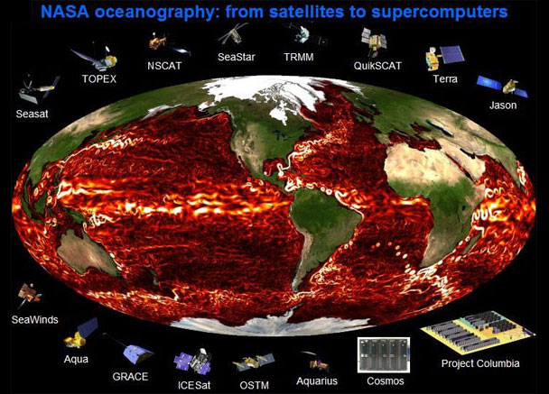
To increase understanding and predictive capability for the ocean's role in future climate change scenarios, the NASA Modeling, Analysis, and Prediction (MAP) program is funding a project called Estimating the Circulation and Climate of the Ocean, Phase II (ECCO2): High-Resolution Global-Ocean and Sea-Ice Data Synthesis. ECCO2 aims to produce increasingly accurate syntheses of all available global-scale ocean and sea-ice data at resolutions that start to resolve ocean eddies and other narrow current systems, which transport heat, carbon, and other properties within the ocean.
ECCO2 data syntheses are obtained by least squares fit of a global full-depth-ocean and sea-ice configuration of the Massachusetts Institute of Technology general circulation model (MITgcm) to the available satellite and in-situ data. ECCO2 data syntheses are being used to quantify the role of the oceans in the global carbon cycle, to understand the recent evolution of the polar oceans, to monitor time-evolving term balances within and between different components of the Earth system, and for many other science applications.
ECCO2 produces increasingly accurate syntheses of all available global-scale ocean and sea-ice data at resolutions that start to resolve ocean eddies and other narrow current systems, which transport heat, carbon, and other properties within the ocean.
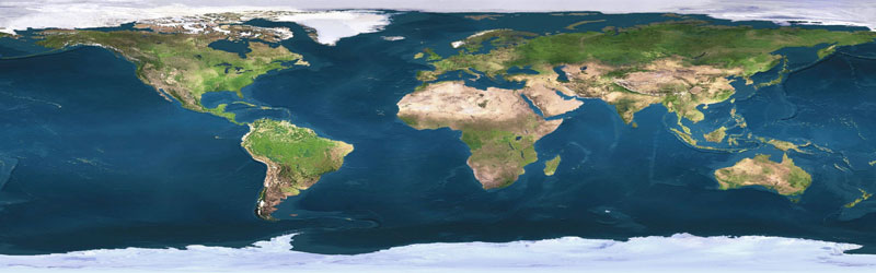
Physical Oceanography (Ozeanographie)
[The contents of this section are from the Open Source Textbook of Robert Stewart, Introduction to Physical Oceanography, 2006. An excellent oceanography textbook.]- Atmospheric Wind Systems
- Wind Driven Ocean Circulation (Sverdrup, Stommel, Munik)
- Observed Circulation in the Atlantic
- Gulf Stream Recirculation Region
The Figure (click to enlarge) shows the distribution of sea-level pressure averaged over the 1979–2001 period. The map shows strong pressure gradients from the west between 40° to 60° latitude, the roaring forties, weaker gradients in the subtropics near 30° latitude, trade-winds from the east in the tropics, and weaker gradients in the east near the Equator. Atmospheric pressure is the result of uneven distribution of solar heating. Wind just above the sea surface is parallel to the contours of constant pressure, and the wind speed is proportional to the gradient of the pressure (spacing of the contours).

Map of mean annual sea-level pressure calculated from the ECMWF 40-year reanalysis. From From Kallberg et al 2005.
What drives the ocean currents? At first, we might answer, the winds drive the circulation. But if we think more carefully about the question, we might not be so sure. We might notice, for example, that strong currents, such as the North Equatorial Countercurrents in the Atlantic and Pacific Oceans go upwind. Spanish navigators in the 16th century noticed strong northward currents along the Florida coast that seemed to be unrelated to the wind. How can this happen? And, why are strong currents found offshore of east coasts but not offshore of west coasts?
Answers to the questions can be found in a series of three remarkable papers published from 1947 to 1951. In the first, Harald Sverdrup (1947) showed that the circulation in the upper kilometer or so of the ocean is directly related to the curl of the wind stress. Henry Stommel (1948) showed that the circulation in oceanic gyres is asymmetric because the Coriolis force varies with latitude. Finally, Walter Munk (1950) added eddy viscosity and calculated the circulation of the upper layers of the Pacific. Together the three oceanographers laid the foundations for a modern theory of ocean circulation.
Sverdrup solutions have been used for describing the global system of surface currents. The solutions are applied throughout each basin all the way to the western limit of the basin. There, conservation of mass is forced by including north-south currents confined to a thin, horizontal boundary layer.
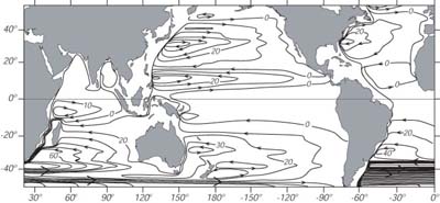 |
| Depth-integrated Sverdrup transport applied globally using the wind stress from Hellerman and Rosenstein (1983). Contour interval is 10 Sverdrups. From Tomczak and Godfrey (1994). |
Observed Circulation in the Atlantic
The theories by Sverdrup, Munk, and Stommel describe a very simple flow. But the ocean is much more complicated. To see just how complicated the flow is at the surface, let's look at a whole ocean basin, the North Atlantic. I have chosen this region because it is the best observed, and because mid-latitude processes in the Atlantic are similar to mid-latitude processes in the other oceans. Thus, for example, we use the Gulf Stream as an example of a western boundary current.
Let's begin with the Gulf Stream to see how our understanding of ocean currents has evolved. Of course, we can't look at all aspects of the flow. You can find out much more by reading Tomczak and Godfrey (1994) book on Regional Oceanography: An Introduction.
North Atlantic Circulation
The North Atlantic is the most thoroughly studied ocean basin. There is an extensive body of theory to describe most aspects of the circulation, including flow at the surface, in the thermocline, and at depth, together with an extensive body of field observations. By looking at figures depicting the circulation, we can learn more about the circulation, and by looking at the figures produced over the past few decades we can trace an ever more complete understanding of the circulation.
Let's begin with the traditional view of the time-averaged flow in the North Atlantic based mostly on hydrographic observations of the density field (Figure 2.8). It is a contemporary view of the mean circulation of the entire ocean based on a century of more of observations. Because the Figure includes all the oceans, perhaps it is overly simplified. So, let's look then at a similar view of the mean circulation of just the North Atlantic (Figure 11.7).
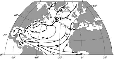 |
| Figure 11.7 Sketch of the major surface currents in the North Atlantic. Values are transport in units of 106m3/s. From Sverdrup, Johnson, and Fleming (1942: fig. 187). |
The figure shows a broad, basin-wide, mid latitude gyre as we expect from Sverdrup's theory described above. In the west, a western boundary current, the Gulf Stream, completes the gyre. In the north a subpolar gyre includes the Labrador current. An equatorial current system and countercurrent are found at low latitudes with flow similar to that in the Pacific. Note, however, the strong cross equatorial flow in the west which flows along the northeast coast of Brazil toward the Caribbean.
If we look closer at the flow in the far north Atlantic (Figure below) we see that the flow is still more complex. This Figure includes much more detail of a region important for fisheries and commerce. Because it is based on an extensive base of hydrographic observations, is this reality? For example, if we were to drop a Lagrangean float into the Atlantic would it follow the streamline shown in the figure?
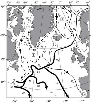 |
Detailed schematic of currents in the North Atlantic showing major surface currents. The numbers give the transport in units on 106m3/s from the surface to a depth of 106m3/s. Eg: East Greenland Current; Ei: East Iceland Current; Gu: Gulf Stream; Ir: Irminger Current; La: Labrador Current; Na: North Atlantic Current; Nc: North Cape Current; Ng: Norwegian Current; Ni: North Iceland Current; Po: Portugal Current; Sb: Spitsbergen Current; Wg: West Greenland Current. Numbers within squares give sinking water in units on 106m3/s. Solid Lines: Relatively warm currents. Broken Lines: Relatively cold currents. From Dietrich, et al. (1980). |
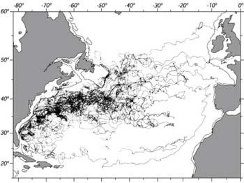
To answer the question, let's look at the tracks of a 110 buoys drifting on the sea surface compiled by Phil Richardson (Figure 11.9 left). The tracks give a very different view of the currents in the North Atlantic. It is hard to distinguish the flow from the jumble of lines, sometimes called spaghetti tracks. Clearly, the flow is very turbulent, especially in the Gulf Stream, a fast, western-boundary current. Furthermore, the turbulent eddies seem to have a diameter of a few degrees. This is much different that turbulence in the atmosphere. In the air, the large eddies are called storms, and storms have diameters of 10° - 20°. Thus oceanic "storms" are much smaller than atmospheric storms.
 |
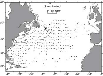 |
Figure Left: Tracks of 110 drifting buoys deployed in the western North Atlantic. Right: Mean velocity of currents in 2° x 2° boxes calculated from tracks above. Boxes with fewer than 40 observations were omitted. Length of arrow is proportional to speed. Maximum values are near 0.6m/s in the Gulf Stream near 37°N 71°W. From Richardson (1981). |
|
Perhaps we can see the mean flow if we average the drifter tracks. What happens when Richardson averages the tracks through 2° x 2° boxes? The averages (Figure up right) begin to show some trends, but note that in some regions, such as east of the Gulf Stream, adjacent boxes have very different means, some having currents going in different directions. This indicates the flow is so variable, that the average is not stable. Forty or more observations do not yields a stable mean value. Overall, Richardson finds that the kinetic energy of the eddies is 8 to 37 times larger than the kinetic energy of the mean flow. Thus the oceanic turbulence is very different than laboratory turbulence. In the lab, the mean flow is typically much faster than the eddies.
Further work by Richardson (1993) based on subsurface buoys freely drifting at depths between 500 m and 3,500 m, shows that the current extends deep below the surface, and that typical eddy diameter is 80 km.
Gulf Stream Recirculation Region
If we look closely at Figure 11.7 (at the top of this section) we see that the transport in the Gulf Stream increases from 26 Sv in the Florida Strait (between Florida and Cuba) to 55 Sv offshore of Cape Hatteras. Later measurements showed the transport increases from 30 Sv in the Florida Strait to 150 Sv near 40°N.
The observed increase, and the large transport off Hatteras, disagree with transports calculated from Sverdrup's theory. Theory predicts a much smaller maximum transport of 30 Sv, and that the maximum ought to be near 28°N. Now we have a problem: What causes the high transports near 40°N?
Niiler (1987) summarizes the theory and observations. First, there is no hydrographic evidence for a large in flux of water from the Antilles Current that flows north of the Bahamas and into the Gulf Stream. This rules out the possibility that the Sverdrup flow is larger than the calculated value, and that the flow bypasses the Gulf of Mexico. The flow seems to come primarily from the Gulf Stream itself. The flow between 60°W and 55°W is to the south. The water then flows south and west, and rejoins the Stream between 65°W and 75°W. Thus, there are two subtropical gyres: a small gyre directly south of the Stream centered on 65°W, called the Gulf Stream recirculation region, and the broad, wind-driven gyre near the surface seen in Figure 11.8 that extends all the way to Europe.
The Gulf Stream recirculation carries two to three times the mass of the broader gyre. Current meters deployed in the recirculation region show that the flow extends to the bottom. This explains why the recirculation is weak in the maps calculated from hydrographic data. Currents calculated from the density distribution give only the baroclinic component of the flow, and they miss the component that is independent of depth, the barotropic component.
The Gulf Stream recirculation is driven by the potential energy of the steeply sloping thermocline at the Gulf Stream. The depth of the 27.00 sigma-theta (σθ ) surface drops from 250 m near 41°N in Figure 10.8 to 800 m near 38°N south of the Stream. Eddies in the Stream convert the potential energy to kinetic energy through baroclinic instability. The instability leads to an interesting phenomena: negative viscosity. The Gulf Stream accelerates not decelerates. It acts as though it were under the influence of a negative viscosity. The same process drives the jet stream in the atmosphere. The steeply sloping density surface separating the polar air mass from mid-latitude air masses at the atmosphere's polar front also leads to baroclinic instability. For more on this topic see Starr's (1968) book on Physics of Negative Viscosity Phenomena.
 |
| Figure 11.10 Gulf Stream meanders lead to the formation of a spinning eddy, a ring. Notice that rings have a diameter of about 1°. From Ring Group (1981). |
Let's look at this process in the Gulf Stream (Figure 11.10). The strong current shear in the Stream causes the flow to begin to meander. The meander intensifies, and eventually the Stream throws off a ring. Those on the south side drift southwest, and eventually merge with the stream several months later (Figure 11.11). The process occurs all along the recirculation region, and satellite images show nearly a dozen or so rings occur north and south of the stream (Figure 11.11). In the south Atlantic, there is another western boundary current, the Brazil Current that completes the Sverdrup circulation in that basin. Between the flow in the north and south Atlantic lies the equatorial circulation similar to the circulation in the Pacific. Before we can complete our description of the Atlantic, we need to look at the Antarctic Circumpolar Current.
 |
| Figure 11.11 Sketch of the position of the Gulf Stream, warm core, and cold core eddies observed in infrared images of the sea surface collected by the infrared radiometer on NOAA-5 in October and December 1978. From Tolmazin (1985: 91). |
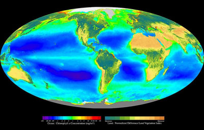 |
Verteilung von Pflanzen in den Ozeanen. (Chlorophyll-Konzentration: Blau = gering, grün = mittel) |
Ökosystem Ozean
Für das Ökosystem Ozean ist das mit zunehmender Tiefe abnehmende Sonnenlicht von großer Bedeutung. Im obersten, vom Sonnenlicht erfüllten Teil des Ozeans, der Euphotischen Zone, nutzen Pflanzen die Photosynthese zur Aufnahme von Energie. Es schließt sich darunter die Disphotische Zone an, wo Sonnenlicht nur noch zum Sehen ausreichend vorhanden ist. In der darunter liegenden Schicht, der Aphotischen Zone, ist kein Sonnenlicht mehr vorhanden.
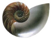
Ein weiteres wichtiges Kennzeichen der Ozeane ist, dass sich das Meereswasser bei unterschiedlichen Tiefen chemisch unterschiedlich verhält. Meereslebewesen, wie beispielsweise Muscheln, Korallen, Kalkalgen und Kieselalgen nutzen Calciumcarbonat und Siliciumdioxid durch Biomineralisation zum Bau von Schalen und Skeletten. Diese Biominerale können allerdings chemisch durch das Meerwasser abgebaut werden. So gibt es für die Calciumcarbonate Aragonit und Calcit (Calcit-Kompensationstiefe) in den Ozeanen eine untere Tiefe, ab der sie sich auflösen.
Der Tiefenverlauf eines Ozeans wird in mehrere Stufen unterteilt. Es beginnt mit dem bis zu 200 m tiefen Schelf. Es schließt sich der Kontinentalhang an, der bis in eine Tiefe von 2000 m bis 3000 m reicht. Dann folgen das Abyssal, welches bis in 6000 m Tiefe reicht, und dann das Hadal.
Zonen des Ozeans
Five depth zones have been identified in the ocean. Life is most abundant in the uppermost ‘euphotic’ layer, where photosynthesis occurs. The mesopelagic is practically dark, and many creatures hide here during the day. The bathypelagic zone begins at 1,000 metres, where the pressure is nearly 100 times greater than at the surface. Below that lies the abyssopelagic zone, down to the sea floor – except where ocean trenches cut through the sea bed, creating what is called a hadopelagic zone.